
Parallel Coordinate Plots with KDEs#
Overlaying kernel density estimation (KDE) plots on a parallel coordinate plot is a helpful way to visualize the distribution of the performance attained for each individual performance objective across all solutions within a Pareto-approximate reference set. KDE plots help:
Illustrate whether there are many alternatives that can achieve a desired performance level, or just a select few
Compare the distribution of performance values across each performance metric for two (or more) distinct sets of solutions.
These plots were first used in Hamilton et al. (2024) and will be demonstrated in the code below. Some of the code is adapted from the paper’s GitHub repository.
An example using parallel coordinate KDE plots#
This example is based off Lau et al. (2023) and shows how the performance tradeoffs of a given solution changes when its decision variables are modestly perturbed.
To plot this figure, let’s begin by importing all the necessary libraries.
import pandas as pd
import numpy as np
import seaborn as sns

import matplotlib.pyplot as plt
from matplotlib import colormaps, cm
from matplotlib.collections import PatchCollection
from matplotlib.patches import Rectangle
from matplotlib.lines import Line2D
from pandas.plotting import parallel_coordinates
import statsmodels.api as sm
---------------------------------------------------------------------------
ModuleNotFoundError                       Traceback (most recent call last)
Cell In[1], line 1
----> 1 import pandas as pd
      2 import numpy as np
      3 import seaborn as sns
      4

ModuleNotFoundError: No module named 'pandas'
Next, let’s define some helper functions (see the GitHub repo they were derived from here) to help plot the parallel coordinate KDE plots.
In the code below, look out for the custom_parallel_coordinates_kde function that implements the parallel coordinate KDE plots.
# function to reorganize and normalize objective data for parallel coordinates plotting
def reorganize_objs(objs, columns_axes, ideal_direction, minmaxs, axis_mins=None, axis_maxs=None):
    """
    Parameters:
        objs (pd.DataFrame): Input dataframe.
        columns_axes (list): List of columns to use as axes.
        ideal_direction (str): 'top' or 'bottom'.
        minmaxs (list): List of 'min' or 'max' for each axis.
        axis_mins (list or None): Optional list of minimum values for each axis.
        axis_maxs (list or None): Optional list of maximum values for each axis.

    Returns:
        objs_reorg (pd.DataFrame): Normalized dataframe.
        tops (list): Top values for each axis.
        bottoms (list): Bottom values for each axis.
    """
    # If min/max directions not given for each axis, assume all should be maximized
    if minmaxs is None:
        minmaxs = ['max'] * len(columns_axes)

    # Get subset of dataframe columns that will be shown as parallel axes
    objs_reorg = objs[columns_axes].copy()

    # Use provided axis min/max or compute from data
    if axis_mins is None:
        axis_mins = objs_reorg.min(axis=0).values
    if axis_maxs is None:
        axis_maxs = objs_reorg.max(axis=0).values

    # Set up tops and bottoms for annotation
    if ideal_direction == 'top':
        tops = axis_maxs.copy()
        bottoms = axis_mins.copy()
    else:
        tops = axis_mins.copy()
        bottoms = axis_maxs.copy()

    # Normalize each axis according to minmaxs and direction
    for i, minmax in enumerate(minmaxs):
        col = objs_reorg.columns[i]
        min_val = axis_mins[i]
        max_val = axis_maxs[i]
        #min_val = objs_reorg[col].min()
        #max_val = objs_reorg[col].max()
        denom = max_val - min_val if max_val != min_val else 1.0
        if ideal_direction == 'top':
            if minmax == 'max':
                objs_reorg[col] = (objs_reorg[col] - min_val) / denom
            else:  # min
                bottoms[i], tops[i] = tops[i], bottoms[i]
                objs_reorg[col] = (max_val - objs_reorg[col]) / denom
        else:  # ideal_direction == 'bottom'
            if minmax == 'max':
                objs_reorg[col] = (max_val - objs_reorg[col]) / denom
            else:  # min
                bottoms[i], tops[i] = tops[i], bottoms[i]
                objs_reorg[col] = (objs_reorg[col] - min_val) / denom

    return objs_reorg, tops, bottoms

### function to get color based on continuous color map or categorical map
def get_color(value, color_by_continuous, color_palette_continuous,
              color_by_categorical, color_dict_categorical):
    if color_by_continuous is not None:
        color = colormaps.get_cmap(color_palette_continuous)(value)
    elif color_by_categorical is not None:
        #print(value)
        color = color_dict_categorical[value]
    return color

### function to get zorder value for ordering lines on plot.
### This works by binning a given axis' values and mapping to discrete classes.
def get_zorder(norm_value, zorder_num_classes, zorder_direction):
    xgrid = np.arange(0, 1.001, 1/zorder_num_classes)
    if zorder_direction == 'ascending':
        return 4 + np.sum(norm_value > xgrid)
    elif zorder_direction == 'descending':
        return 4 + np.sum(norm_value < xgrid)

### customizable parallel coordinates plot
# Adapted from Figure 5 of Hamilton et al 2024 (source: https://www.nature.com/articles/s41467-024-51660-8)
def custom_parallel_coordinates_kde(fig, ax, objs, columns_axes=None, axis_labels=None,
                                ideal_direction='top', minmaxs=None,
                                zorder_by=None, zorder_num_classes=10, zorder_direction='ascending',
                                color_original='red', color_ptb='coral',
                                alpha_original=0.8, alpha_ptb=0.4,
                                lw_original=3, lw_ptb=1.5, fontsize=14,
                                axis_mins=None, axis_maxs=None):

    ### verify that all inputs take supported values
    assert ideal_direction in ['top','bottom']
    assert zorder_direction in ['ascending', 'descending']

    if minmaxs is not None:
        for minmax in minmaxs:
            assert minmax in ['max','min']

    if columns_axes is None:
        columns_axes = objs.columns
    if axis_labels is None:
        axis_labels = columns_axes

    objs_original = objs[objs['Category'] == 'original'].reset_index(drop=True)
    objs_ptb = objs[objs['Category'] == 'perturbations'].reset_index(drop=True)

    ### reorganize & normalize objective data
    objs_reorg_ptb, tops_ptb, bottoms_ptb = reorganize_objs(objs_ptb, columns_axes, ideal_direction,
                                                            minmaxs, axis_mins=axis_mins, axis_maxs=axis_maxs)
    objs_reorg_original, tops_original, bottoms_original = reorganize_objs(objs_original, columns_axes,
                                                                           ideal_direction, minmaxs,
                                                                           axis_mins=axis_mins, axis_maxs=axis_maxs)

    ### loop over all solutions/rows & plot on parallel axis plot
    for j in range(objs_reorg_original.shape[1]-1):
        y = [objs_reorg_original.iloc[0, j], objs_reorg_original.iloc[0, j+1]]
        x = [j, j+1]
        ax.plot(x, y, c=color_original, alpha=alpha_original, zorder=4+1, lw=lw_original)

    for i in range(objs_reorg_ptb.shape[0]):
        ### order lines according to ascending or descending values of one of the objectives?
        if zorder_by is None:
            zorder = 4
        else:
            zorder = get_zorder(objs_reorg_ptb[columns_axes[zorder_by]].iloc[i],
                                zorder_num_classes, zorder_direction)

        ### loop over objective/column pairs & plot lines between parallel axes
        for j in range(objs_reorg_ptb.shape[1]-1):
            y = [objs_reorg_ptb.iloc[i, j], objs_reorg_ptb.iloc[i, j+1]]
            x = [j, j+1]
            ax.plot(x, y, c=color_ptb, alpha=alpha_ptb, zorder=0, lw=lw_ptb)

    ### add top/bottom ranges
    for j in range(len(columns_axes)):
        ax.annotate(str(round(tops_ptb[j],3)), [j, 1.02], ha='center', va='bottom',
                    zorder=2, fontsize=fontsize)
        if j == len(columns_axes)-1:
            ax.annotate(str(round(bottoms_ptb[j],3)) + '+', [j, -0.02], ha='center', va='top',
                        zorder=2, fontsize=fontsize)
        else:
            ax.annotate(str(round(bottoms_ptb[j],3)), [j, -0.02], ha='center', va='top',
                        zorder=2, fontsize=fontsize)

        ax.plot([j,j], [0,1], c='k', zorder=1)

    # add distribution of perturbed objectives
    for j in range(len(columns_axes)):
        data = objs_reorg_ptb[columns_axes[j]]
        data_scaled = data
        kde = sm.nonparametric.KDEUnivariate(data_scaled)
        kde.fit(bw=0.025)

        y = np.arange(0, 1.01, 0.01)
        x = []
        for yy in y:
            xx = kde.evaluate(yy) * 0.095
            if np.isnan(xx):
                x.append(0.)
            else:
                x.append(xx[0])
        x = np.array(x)
        # ensure that the KDE filled area is plotted over the lines
        ax.fill_betweenx(y+0.075, x + j, j, where=(x > 0.00005), lw=1, alpha=0.65, zorder=600, fc=color_ptb, ec='k')

    ### other aesthetics
    ax.set_xticks([])
    ax.set_yticks([])

    for spine in ['top','bottom','left','right']:
        ax.spines[spine].set_visible(False)

    if ideal_direction == 'top':
        ax.arrow(-0.15,0.1,0,0.7, head_width=0.08, head_length=0.05, color='k', lw=1.5)
    elif ideal_direction == 'bottom':
        ax.arrow(-0.15,0.9,0,-0.7, head_width=0.08, head_length=0.05, color='k', lw=1.5)
    ax.annotate('Direction of preference', xy=(-0.3,0.5), ha='center', va='center',
                rotation=90, fontsize=fontsize)

    ax.set_xlim(-0.4, len(columns_axes)+0.3)
    ax.set_ylim(-0.4,1.1)

    for i,l in enumerate(axis_labels):
        ax.annotate(l, xy=(i,-0.12), ha='center', va='top', fontsize=fontsize)
    ax.patch.set_alpha(0)


### customizable parallel coordinates plot
def single_parallel_coordinates(fig, ax, objs, columns_axes=None, axis_labels=None,
                                ideal_direction='top', minmaxs=None,
                                color_by_categorical=None, color_palette_categorical=None, color_dict_categorical=None,
                                zorder_by=None, zorder_num_classes=10, zorder_direction='ascending',
                                alpha_base=0.8, lw_base=1.5, fontsize=14, save_fig_filename=None,
                                axis_mins=None, axis_maxs=None):

    ### verify that all inputs take supported values
    assert ideal_direction in ['top','bottom']
    assert zorder_direction in ['ascending', 'descending']

    if minmaxs is not None:
        for minmax in minmaxs:
            assert minmax in ['max','min']

    if columns_axes is None:
        columns_axes = objs.columns
    if axis_labels is None:
        axis_labels = columns_axes

    ### reorganize & normalize objective data
    objs_reorg, tops, bottoms = reorganize_objs(objs, columns_axes, ideal_direction, minmaxs,
        axis_mins=axis_mins, axis_maxs=axis_maxs)

    ### loop over all solutions/rows & plot on parallel axis plot
    for i in range(objs_reorg.shape[0]):
        sol_i_cat = objs.iloc[i][color_by_categorical]
        color = color_dict_categorical[sol_i_cat]

        ### order lines according to ascending or descending values of one of the objectives?
        if zorder_by is None:
            zorder = 0
        else:
            zorder = get_zorder(objs_reorg[columns_axes[zorder_by]].iloc[i],
                                zorder_num_classes, zorder_direction)
        alpha = alpha_base
        lw = lw_base

        ### loop over objective/column pairs & plot lines between parallel axes
        for j in range(objs_reorg.shape[1]-1):
            y = [objs_reorg.iloc[i, j], objs_reorg.iloc[i, j+1]]
            x = [j, j+1]
            ax.plot(x, y, c=color, alpha=alpha, zorder=zorder, lw=lw)

def get_objs_util(objs_df, util):
    objs_util_df = objs_df[[col for col in objs_df.columns if col.endswith(f'_{util[0]}')]]
    return objs_util_df
Import the required datasets#
In this example, we have three hypothetical utilities: Watertown (W), Dryville (D) and Fallsland (F). Each utility have five performance objectives to meet:
Reliability (REL)
Restriction frequency (RF)
Infrastructure Net Present Cost (INPC)
Peak financial cost (PFC)
Drought mitigation cost (DMC)
# original solution colors
color_sol1 = "#B66D0D"
color_sol2 = "#34563A"

# perturbed solution colors
color_sol1_ptb = "#EACCA4"
color_sol2_ptb = "#B9DFC7"

# the different objectives and utilities
objs_names = ['REL', 'RF', 'INPC', 'PFC', 'WCC']
util_names = ['Watertown', 'Dryville', 'Fallsland']
util_dict = {0: 'Watertown', 1: 'Dryville', 2: 'Fallsland'}

# create a list of all objective names for all utilities
objs_names_allutils = [obj_name + '_' + util_name[0] for util_name in util_names for obj_name in objs_names]

obj_names_W = ['REL_W', 'RF_W', 'INPC_W', 'PFC_W', 'WCC_W']
obj_names_D = ['REL_D', 'RF_D', 'INPC_D', 'PFC_D', 'WCC_D']
obj_names_F = ['REL_F', 'RF_F', 'INPC_F', 'PFC_F', 'WCC_F']

# create a dictionary to map utility names to their corresponding objective names
obj_names_dict = {'W': obj_names_W, 'D': obj_names_D, 'F': obj_names_F}
Once the utilities and their respective performance objectives have been specified, let’s load the data for the perturbed solutions.
# get the perturbed versions of the solutions without regional values
objectives_ptb_sol1 = pd.read_csv(f'example_data/objs_ptb_set1.csv',
                                     index_col=None, header=None)
objectives_ptb_sol1.columns = objs_names_allutils
objectives_ptb_sol2 = pd.read_csv(f'example_data/objs_ptb_set2.csv',
                                       index_col=None, header=None)
objectives_ptb_sol2.columns = objs_names_allutils

# create categories for the perturbed solutions for plotting
objectives_perturbed_sol1_cat = objectives_ptb_sol1.copy()
objectives_perturbed_sol1_cat['Category'] = 'perturbations'
objectives_perturbed_sol2_cat = objectives_ptb_sol2.copy()
objectives_perturbed_sol2_cat['Category'] = 'perturbations'
Similarly, we can upload the performance tradeoffs of the original solutions.
# read in the original objectives for the two solutions
objectives_original = pd.read_csv(f'example_data/objectives_original.csv', index_col=None,
                                  header=None, names=objs_names_allutils)

objectives_og_sol1 = pd.DataFrame(objectives_original.iloc[0, :]).T
objectives_og_sol2 = pd.DataFrame(objectives_original.iloc[1, :]).T

# create categories for the orignal solutions for plotting
objectives_og_sol1_cat = objectives_og_sol1.copy()
objectives_og_sol1_cat['Category'] = 'original'
objectives_og_sol2_cat = objectives_og_sol2.copy()
objectives_og_sol2_cat['Category'] = 'original'
Let’s combine the two sets of solutions so we can plot them.
# combine the perturbed and original versions of the solutions
objectives_sol1_combined_cat = pd.concat((objectives_perturbed_sol1_cat, objectives_og_sol1_cat), ignore_index=True)
objectives_sol2_combined_cat = pd.concat((objectives_perturbed_sol2_cat, objectives_og_sol2_cat), ignore_index=True)
Plot the parallel tradeoffs#
Here, we first select a utility to plot using the util_to_plot variable
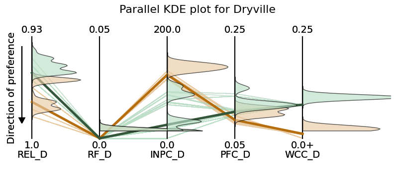
This is how you can interpret figure:
The KDE plots show the distribution of performance tradeoffs of each perturbed instance of a solution.
The solid, thick line shows the original performance tradeoffs of the solution
The thinner, slightly transparent lines show the performance tradeoff of each perturbed instance of the solution.
But first, let’s set up the datasets and figure specifications we want to plot.
# specify the utility to plot
util_to_plot = "Dryville"

# get the objectives for the original and perturbed solutions for plotting
objs_to_plot_sol1 = get_objs_util(objectives_sol1_combined_cat.drop(columns=['Category']), util_to_plot)
objs_to_plot_sol1['Category'] = objectives_sol1_combined_cat['Category']

objs_to_plot_sol2 = get_objs_util(objectives_sol2_combined_cat.drop(columns=['Category']), util_to_plot)
objs_to_plot_sol2['Category'] = objectives_sol2_combined_cat['Category']

# specify the axis min and max values for the parallel coordinates plot
axis_mins = [0.93, 0.0, 0.0, 0.05, 0.0]
axis_maxs = [1.0, 0.05, 200.0, 0.25, 0.25]

# get the axis labels (all but the last Category column) for the parallel coordinates plot
columns_axes = objs_to_plot_sol1.drop(columns=['Category']).columns
axis_labels = columns_axes
Dryville’s performance tradeoffs#
Let’s take a look at how modest perturbations to Watertown’s decision variables change its performance tradeoffs.
# setup figure specifications and dimensions
figsize = (10,4)
fontsize = 14

fig, ax = plt.subplots(1,1,figsize=figsize, gridspec_kw={'hspace':0.1, 'wspace':0.1})

custom_parallel_coordinates_kde(fig, ax, objs_to_plot_sol1, columns_axes=columns_axes, axis_labels=axis_labels,
                                ideal_direction='bottom', minmaxs=['max','min','min','min','min'],
                                color_original=color_sol1, color_ptb=color_sol1_ptb,
                                alpha_original=1.0, alpha_ptb=0.075,
                                lw_original=3.5, lw_ptb=1.0, fontsize=14,
                                axis_mins=axis_mins, axis_maxs=axis_maxs)

custom_parallel_coordinates_kde(fig, ax, objs_to_plot_sol2, columns_axes=columns_axes, axis_labels=axis_labels,
                                ideal_direction='bottom', minmaxs=['max','min','min','min','min'],
                                color_original=color_sol2, color_ptb=color_sol2_ptb,
                                alpha_original=1.0, alpha_ptb=0.075,
                                lw_original=3.5, lw_ptb=1.0, fontsize=14,
                                axis_mins=axis_mins, axis_maxs=axis_maxs)

ax.set_title(f'Parallel KDE plot for {util_to_plot}', fontsize=fontsize+2, pad=20)
plt.show()
Feel free to try this out with Watertown and Fallsland as well! Be careful to make the necessary modifications to the figure specifications before plotting to get the best result.
Conclusion#
This example provides a guideline on how to plot a figure that combines both KDE plots and parallel coordinate plots. If you have any suggestions to improve this style of figure, feel free to open a GitHub Issue or contribute directly to this page in the Reed Group Lab Manual repository.